Linear Regression
TOC
Introduction
This is the hello world of econometrics and machine learning. Before diving into the mathematical equations, let’s make some terms clear with an example. First, since there is a function, we would use it to map input into output. Output is the desired variable such as the price of a house that we would like to predict. Input would be the features of that house such as: age, floors, rooms, location, etc. If we have information about many houses, we can perform a linear regression on that dataset. The linear regression function would use one parameter per input to take into account the information that input carries so that the meaning of the input (age) carries over into the output.
To understand what the name linear regression means: it is linear since the addition of the multiplication of parameters and inputs are linear operations. It is regression since it outputs a predicted value (the symbol y is with a hat). Here is the mathematical function:
\[\hat{y} = \theta_{0} + \theta_{1} x_{1} + \theta_{2} x_{2} + ... + \theta_{n} x_{n}\]with n is the number of features, \(x_{i}\) is the \(i_{th}\) feature value, \(\theta_{j}\) is the \(j_{ith}\) model parameter (\(\theta_{0}\) is the bias term and \(\theta_{1}, \theta_{2},...,\theta_{n}\) are feature weights. There is a vector form for it:
\[\hat{y}=h_{\theta}(x) = \theta \cdot x\]Where \(h_{\theta}\) is the hypothesis function with parameter vector .
Linear regression is among the parts of machine learning that reuses traditional econometrics (others include Bayesian inference, Maximum Likelihood). It is reused since the problem remains evergreen: given a dataset, how to find the fittest relationship that fits inputs x into the output y. To explain in better words: we care about some character y of a second hand car the most - in this case y is the price, therefore we collect and select data of its features (mileage, age, brand). With that dataset, we use mathematics to find the best possible function that maps from the input vector into its price. When we say best possible, we mean to reduce some sort of distance of the real ys and the computed function to the least. Still in traditional econometrics, the distance (also called error) is the Euclidean distance between the point y and the line. Then we take average and it is called mean square error (MSE), with \(x^{(i)}\) to be the vector of x at \(i^{th}\) instance, and X to denote the matrix containing all feature vectors of all instances in the dataset excluding labels y column vector:
\[MSE (X, h_{\theta}) = \frac{1}{m} \sum_{i=1}^{m} (\theta^{\top} x^{(i)} -y^{(i)})^{2} = \frac{1}{m} ||y - X \theta ||_{2}^{2}\]Since X and h are known, the problem becomes finding to min MSE: \(\theta^{*} = arg min_{\theta} MSE(\theta)\). To minimize MSE, firstly, there is a closed form solution. A closed form solution is a solution derived by mathematical logic with mathematical symbols in it. An analytical solution is a solution by giving numerical values to prove its quality of solving the problem. Here is how to derive the closed form solution: we solve the optimization problem by letting its gradient be 0. For a linear model, this is straightforward: we compute the partial derivatives of the cost function with regard to the parameter j, then we put them all together in a big notation. Partial gradient by j of the error function is calculated using chain rule:
\[\frac{\partial}{\partial \theta_{j}}MSE(\theta) = \frac{1}{m} \sum_{i=1}^{m} 2(\theta^{\top} x^{(i)} - y^{(i)}). \frac{\partial}{\partial \theta_{j}}(\theta^{\top} x^{(i)} - y^{(i)})\] \[= \frac{2}{m} \sum_{i=1}^{m}(\theta^{\top} x^{(i)} - y^{(i)}) x_{j}^{(i)} \forall j \in (1,n)\]Sometimes they put a \(\frac{1}{2}\) as a multiplicator in MSE to cancel out the scalar 2, for convenient. The gradient by \(\theta\) of the error function in the vector notation would be:
\[\nabla_{\theta}MSE(\theta){\partial \theta} = \frac{2}{m} X^{\top} (X \theta - y) = 0\] \[\Leftrightarrow X^{\top} X \theta = X^{\top} y\] \[\Leftrightarrow = (X^{\top} X)^{-1} X^{\top} y\](this is known as the normal equation)
Apart from MSE, we use some other function that fits our modern purpose in some other way. And we call that class of functions cost function (or loss function). To show an example, another useful loss function is MAE (mean absolute error):
\[MAE (X, h) = \frac{1}{m} \sum_{i=1}^{m} | h(x^{(i)}) - y^{(i)} |\]We can see that, instead of taking the Euclidean norm, it just minus the real y from the predicted value y and takes the positive value of that difference. With the square and square root way of calculation, the RMSE is more sensitive to outliers.
In the next section, we look at the second approach to find the minimum: using gradient descent as a search algorithm.
Gradient descent
In econometrics, if we can approximate the distribution of the population by estimating the parameters of the function of the sample data then we are done. Since the sample is the representative part of the population. Voila, we found and are now able to describe the interested population well. For example: we have the population of smokers in a given region of the world, then we can suggest policy in the direction of improving people’s health in that region. In machine learning, however, the purpose is different since we are somewhat closer to the market: we need to generate predictions and those predictions need to be good enough. In other words, the algorithm needs to work well on unseen data (unforeseen future). We also live in an era where the dataset has become big - so big at the scale that researchers haven’t seen before. Together with the technological advance that gives us computing resources a lot more freedom than in decades ago - at the beginning of machine learning conception. With that in mind, we can continue to explore machine learning as a powerful and pragmatic tool in the modern world, at the same time keeping mathematics and other closely related fields in our toolbelt.
One of the highlights of this modern field is that we use an optimization approach called gradient descent to iteratively change parameters to minimize the loss function. And we use Python. Imagine a general function of any shape (with mountains and valleys). The gradient descent is a technique that guides along the slope of the graph (assumed loss function) until it reaches a minimum.
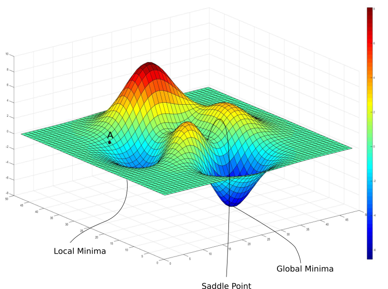
Source: https://blog.paperspace.com/intro-to-optimization-in-deep-learning-gradient-descent/
Assume that the above terrain is a loss function’s graph, when we see it and ask the question how to achieve that minimum, we can come up with the following procedure:
- Randomly initialize the parameters/weights $$ \theta $$ .
- Since we need to move in the direction of the steepest possible descent (hence the name), we update the parameter vector with: $$ \theta_{j} \leftarrow \theta_{j} - \alpha \frac{\partial}{\partial \theta_{j}} Loss(\theta), \forall j \in (1,n) $$ (we descend by one parameter/dimension at a time). This is equivalent to: $$ \theta \leftarrow \theta - \alpha \frac{\partial}{\partial \theta}Loss(\theta) $$
- Stop when converged
Full gradient descent takes into account the full training dataset, but it is computationally costly. Another way to do it is to take into account only a mini batch of the training set each time. Stochastic gradient descent is when the algorithm takes into account only one instance of the training data at a time.
Notice that \(\alpha\) can be tuned to be constant (usually at 0.1) or it can be adaptive (\(\alpha = \frac{1}{\text{updates so far}}\)).
Maximum likelihood
This is also a classical technique to demonstrate that the loss function of least squares is a natural and obvious implication of the linear regression model.
Back to the linear equation, this time with an error term (this is econometrics!)
\[y^{(i)} = \theta^{\top} x^{(i)}+ \epsilon^{(i)}\]\(\epsilon\) contains both unknown inputs and random noise. For this technique, we need to assume \(\epsilon^{(i)}\) are iid (independently and identically distributed) according to a Gaussian distribution with mean 0 and variance \(\sigma^{2}\).
\[p(\epsilon^{(i)}) = \frac{1}{\sqrt{2\pi} \sigma} exp(-\frac{(\epsilon^{(i)})^{2}}{2 \sigma^{2}})\] \[\Rightarrow p(y^{(i)}|x^{(i)};\theta)=\frac{1}{\sqrt{2\pi}\sigma}exp(-\frac{(y^{(i)}-\theta^{\top} x^{(i)})^{2}}{2\sigma^{2}})\]We need to find a way to maximize the probability of y that was given in relation with x and \(\theta\). This way involves finding parameters, hence we can rewrite:
\[L(\theta) = L(\theta;X,y) = p(y|X;\theta)\]This is to find \(\theta\) that maximize the joint distribution of X (so that y happens the most):
\[L(\theta) = \prod_{i=1}^{n} p(y^{(i)}|x^{(i)};\theta) = \prod_{i=1}^{n} \frac{1}{\sqrt{2\pi}\sigma} exp(-\frac{(y^{(i)} - \theta^{\top} x^{(i)})^{2}}{2\sigma^{2}})\]Maximizing \(L(\theta)\) is similar to maximizing the log likelihood:
\[l(\theta) = log L(\theta) = log \prod_{i=1}^{n} \frac{1}{\sqrt{2\pi}\sigma} exp(-\frac{(y^{(i)} - \theta^{\top} x^{(i)})^{2}}{2\sigma^{2}})\] \[= \sum_{i=1}^{n} log \frac{1}{\sqrt{2\pi}\sigma} exp(-\frac{(y^{(i)} - \theta^{\top} x^{(i)})^{2}}{2\sigma^{2}})\]\(= n log \frac{1}{\sqrt{2\pi}\sigma} - \frac{1}{\sigma^{2}} \frac{1}{2} \sum_{i=1}^{n}(y^{(i)} - \theta^{\top} x^{(i)})^{2}\) Taking out all the scalar values in the above function, we have MSE. It means that when we find the maximum likelihood of \(\theta\) for maximizing the joint probability of X, we come to the least square error function. That’s it for econometrics!
Non-linear linear
When we add a quadratic term of x, if the parameters \(\theta\) still come together as a linear combination, the problem can still be solved as a linear regression in general. Note that, the nature of feature x changes since it becomes a nonlinear input. Nonlinear input or nonlinear combination of input can address better and more complex relationship in the data. This is called feature engineering in which we found a special subset of features that explain the output better than each of those in separate.
Code
Let’s explore a housing dataset, we have eight factors (median income, bedsroom, house age, average population, etc) and the target to be house value. In machine learning, before doing model training, we split the dataset into a training and a test set, usually at 80-20 rule. The training is to fit the parameters and the test set is to validate/test those parameters. This gives us a sense of unseen data. It prepares us for the unforeseen but incoming data so that when we do all the calculation for the algorithm, we keep in mind the aim to predict the future as good as possible.
!pip install sklearn
Requirement already satisfied: sklearn in /Users/nguyenlinhchi/opt/anaconda3/lib/python3.9/site-packages (0.0.post1)
from sklearn.datasets import fetch_california_housing
from sklearn.preprocessing import StandardScaler
from sklearn import linear_model
import matplotlib.pyplot as plt
import seaborn as sns
import numpy as np
import pandas as pd
from sklearn.model_selection import train_test_split
from sklearn.metrics import mean_squared_error, r2_score
california_housing = fetch_california_housing(as_frame=True)
california_housing.data.head()
| MedInc | HouseAge | AveRooms | AveBedrms | Population | AveOccup | Latitude | Longitude | |
|---|---|---|---|---|---|---|---|---|
| 0 | 8.3252 | 41.0 | 6.984127 | 1.023810 | 322.0 | 2.555556 | 37.88 | -122.23 |
| 1 | 8.3014 | 21.0 | 6.238137 | 0.971880 | 2401.0 | 2.109842 | 37.86 | -122.22 |
| 2 | 7.2574 | 52.0 | 8.288136 | 1.073446 | 496.0 | 2.802260 | 37.85 | -122.24 |
| 3 | 5.6431 | 52.0 | 5.817352 | 1.073059 | 558.0 | 2.547945 | 37.85 | -122.25 |
| 4 | 3.8462 | 52.0 | 6.281853 | 1.081081 | 565.0 | 2.181467 | 37.85 | -122.25 |
X = california_housing.data
y = california_housing.target
# Scale the dataset, since it has wildly different ranges
scaler = StandardScaler()
X_scaled = scaler.fit_transform(X)
# concatnate y so that we have a correlation matrix
# what correlates the most to y (house price) is median income

# from pandas.plotting import scatter_matrix
# scatter_matrix(data, figsize=(12, 8))
# plt.show()

y_new=np.array(y).reshape(-1,1)
data=np.append(X_scaled, y_new, axis=1)
data=pd.DataFrame(data)
sns.pairplot(data)
plt.show()


# train a linear regression model
X_train, X_test, y_train, y_test = train_test_split(X_scaled, y, test_size=0.2, random_state=42)
regr = linear_model.LinearRegression()
regr.fit(X_train,y_train)
# the most importance factor is median income
# second is the average bedrooms
print(regr.coef_)
y_pred=regr.predict(X_test)
# MSE is 0.56 and R square is 0.57 (an econometrics indicator of
# how much explaination power of this model with regard to the
# whole dataset)
print(mean_squared_error(y_test, y_pred))
print(r2_score(y_test,y_pred))
[ 0.85238169  0.12238224 -0.30511591  0.37113188 -0.00229841 -0.03662363
 -0.89663505 -0.86892682]
0.555891598695244
0.5757877060324511
# with max y_test of 5, a MSE of 0.55 is considered to be good
max(y_test)
5.00001
# plot y_test and y_pred wrt median income
# we have 0.5 MSE which is good enough
plt.scatter(X_test[:,0], y_test, color="black")
plt.plot(X_test[:,0], y_pred, color="blue", linewidth=1)
plt.xticks(())
plt.yticks(())
plt.show()


def gradient_descent(W, x, y):
    y_hat = x.dot(W).flatten()
    error = (y - y_hat)
    mse = (1.0 / len(x)) * np.sum(np.square(error))
    gradient = -(1.0 / len(x)) * error.dot(x)
    return gradient, mse
w = np.array((10,10,10,10,10,10,10,10))
alpha = .1
tolerance = 1e-3
old_w = []
errors = []
# Gradient Descent
iterations = 1
for i in range(200):
    gradient, error = gradient_descent(w, X_scaled, y)
    new_w = w - alpha * gradient

    # Print error every 10 iterations
    if iterations % 10 == 0:
        print("Iteration: %d - Error: %.4f" % (iterations, error))
        old_w.append(new_w)
        errors.append(error)

    # Stopping Condition
    if np.sum(abs(new_w - w)) < tolerance:
        print('Gradient Descent has converged')
        break

    iterations += 1
    w = new_w

print('w =', w)
Iteration: 10 - Error: 87.8141
Iteration: 20 - Error: 29.5025
Iteration: 30 - Error: 18.4665
Iteration: 40 - Error: 15.1451
Iteration: 50 - Error: 13.5619
Iteration: 60 - Error: 12.4791
Iteration: 70 - Error: 11.6017
Iteration: 80 - Error: 10.8480
Iteration: 90 - Error: 10.1882
Iteration: 100 - Error: 9.6070
Iteration: 110 - Error: 9.0935
Iteration: 120 - Error: 8.6392
Iteration: 130 - Error: 8.2366
Iteration: 140 - Error: 7.8793
Iteration: 150 - Error: 7.5620
Iteration: 160 - Error: 7.2797
Iteration: 170 - Error: 7.0284
Iteration: 180 - Error: 6.8043
Iteration: 190 - Error: 6.6042
Iteration: 200 - Error: 6.4255
w = [ 1.82152727  0.51084912 -1.75407177  1.36706096  0.12526811 -0.093646
  2.88974467  2.82229194]
# compare to the model calculated by sklearn
regr.coef_
array([ 0.85238169,  0.12238224, -0.30511591,  0.37113188, -0.00229841,
       -0.03662363, -0.89663505, -0.86892682])